Blog 3: Design of Experiments
- nicholasleejh05
- Jan 31, 2025
- 18 min read
Updated: Feb 1, 2025
Hey you, miss me? It's been 8 weeks since my last blog and it's time for another one. Buckle up because I have so many things to share, but first, recap time!
In my second blog, I shared my experience with Arduino Programming, from when I didn't enjoy it because of my experience in 2022 when I used a Micro bit to now which I find programming more fun. In this blog, I will introduce to you design of experiments! With that, let's jump right into it!
Design of Experiments
Before we get into the juicy part of the blog, I didn't expect myself to be learning design of experiment as I didn't knew it existed before. However, I was surprised to learn that I have used it before in one of my practical modules Laboratory and Process Skills 2 where I identify the optimal process parameters to extract the highest amount of coffee soluble from roasted coffee beans. Hence, I knew that this topic will be very useful for my final year project.
Moving forward, we first need to understand what design of experiments is all about. A design of experiments is a statistics-based approach to design experiments and optimizing the experimental process itself. It is also a methodology to obtain knowledge of a complex, multi-variable process with the fewest trials possible. Hence, making it the backbone of any product design as well as any process or product improvement efforts. Our goal by using the design of experiments is to understand the process by determining which factors are most influential on the output. (Yes it's from the presentation slides)
You might be wondering why should we use design of experiments? And that is a very good question! Imagine a scenario where your boss wants you to investigate the loss of popcorn yield. Additionally, 3 factors were identified that affects the popcorn yield which are diameter of bowls to contain the corn, microwaving time and power setting of microwave. Moreover, there are two factors and there is a need to replicate 8 times. This means that you need to conduct a total amount of 64 experiments. The total amount of experiments can be determined by using the equation down below.

However, conducting 64 experiments will result in a huge loss of popcorn as well as time. Hence, making it inefficient and resource-ineffective. One way to achieve similar result is to use fractional factorial design which reduces the total number of experiments down to 32. Hence, the design of experiments can help us study the effects, minimizing both time and resources. This example is the assignment that I was given that I will explain in depth below. Now that we have understood what is design of experiment is, let's move onto the next part!
Assignment
Now that you have understood what is design of experiment is and their advantages, it's time for the juicy part of the blog! I was recently given an assignment or case study based on popcorn example above. The objectives and data are listed down below:
Full Factorial
Determine the effect of single factors and their ranking.
Determine the interaction effects.
Include all tables and graphs.
Include the conclusion of the data analysis.
Fractional Factorial
Determine the effect of single factors and their ranking.
Include all tables and graphs.
Include the conclusion of the data analysis.

Since my admission number ended with 74, this will be my data as shown above.
Factors and levels (-) or (+) that affects popcorn yield:
Factor A: Diameter of bowls to contain corn [10cm (-) and 15cm (+)]
Factor B: Microwaving time [4minutes (-) and 6minutes (+)]
Factor C: Power setting of microwave [75% (-) and 100% (+)]
Now that we have the objective and data, let's move onto the next part of the blog!
Full Factorial Design
To prove my point that design of experiments is able to save both resources and time, I will be doing both full and fractional factorial design. However, I will do the full factorial design first followed by fractional factorial design.
Before we can determine the effect of each factor, we have to do some calculations first for each factor and levels as shown down below.

This calculation allow us to determine the average value for a specific factor and level. For example, we add up all of the runs where factor A is high which are run order 1,4,5 and 6. We also add up all of the runs where factor A is low which are run order 2,3,7 and 8. By doing so, we are able to average the other factors which are B and C. Hence, we are able to determine the effect of changing factor A which is the diameter changes from 10cm to 15cm. In conclusion, this step is to help us determine the effect of a single factor when the level changes from high to low.
With the calculations completed, we can now create our chart and graph as shown below. It's time to determine the effects of a single factors and their rankings!

With the chart created, we can observe the effects for each factor:
Factor A: When the diameter of the bowl increases from 10cm to 15cm, the mass of bullets decreases from 1.84g to 1.69g.
Factor B: When the microwaving time increases from 4minutes to 6 minutes, the mass of bullets decreases from 2.14g to 1.39g.
Factor C: when the power setting of microwave increases from 75% to 100%, the mass of bullets decreases from 2.84g to 0.69g.
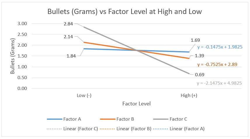
To determine the rankings of the factor that has the most to least significant impact on the mass of bullets, we must look at the factor with the steepest gradient. The greater the gradient coefficient, the more significant the factor affects the mass of bullets.
From the graph above, it can be shown that the ranking of the factors are:
Factor C: Power setting of the microwave is the most significant factor with the largest gradient coefficient of 2.1475.
Factor B: Microwaving time is the next most significant factor with the second highest gradient coefficient of 0.7525.
Factor A: Diameter of bowl is the least significant factor with the lowest gradient coefficient of 0.1475.
Now that we have determine the rankings of the factors, it's time to determine the interaction effects. For example, the boiling point of a matter is dependent on both temperature and pressure. Hence, it's is an important step to determine whether two factors are interacting with each other. To do so, we have to do another calculations as shown below.
Calculating for A x B:

This calculations will allow us to create a table as shown below which is necessary to create our graph.

From the table above, it can be seen that when factor A is low and factor B level increases from low to high, the mass of bullets decreases from 1.93g to 1.74g. Additionally, when factor A is high and factor B level increases from low to high, the mass of bullets significantly decreases from 2.74g to 1.03g. However, the graph below shows a better way to analyze data.

To determine whether there are interaction between both factors, one have to also look at the gradient. The greater the difference in gradient, the larger the interaction between both factors. From the graph above, it can be seen that both lines are negative and of different values which are -0.19 and -1.71. Hence, there's a significant interaction between A and B. With A x B completed, it's time to repeat the same steps for A x C and B x C.
Calculating for A x C:

Similarly, this calculations will allow us to create a table as shown below which is necessary to create our graph.

Looking at the table, it can be shown that when factor A is low and factor C level increases from low to high, the mass of bullets decreases significantly from 2.93g to 0.74g. Similarly, as factor A is high and factor C level increases from low to high, the mass of bullets decreases significantly from 2.74g to 0.64g. However, the graph below shows a better way to analyze data.

As previously mentioned, to determine whether there are interaction between both factors, one have to also look at the gradient. The greater the difference in gradient, the larger the interaction between both factors. From the graph above, it can be seen that the gradients of both lines are different by a little margin which are -2.19 and -2.105. Hence, there's a small interaction between A and C. Lastly, it's time to repeat the steps for B x C.
Calculating for B x C:

Similarly, this calculations will allow us to create a table as shown below which is necessary to create our graph.

Looking at the table above, it can be seen that when factor B is low and factor C level increases from low to high, the mass of bullets decreases significantly from 3.43g to 0.85g. Similarly, when factor B is high and factor C increases from low to high, the mass of bullets decreases from 2.24g to 0.53g. However, the graph below shows a better way to analyze data.
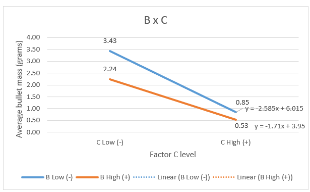
As previously mentioned again, to determine whether there are interaction between both factors, one have to also look at the gradient. The greater the difference in gradient, the larger the interaction between both factors. From the graph above, it can be seen that both lines are negative and of different values which are -2.585 and -1.71. Hence, there's a significant interaction between B and C.
Findings
Now that we have analyze our data, it's time to summarize our findings!
Increasing the factor levels for any factor will result in a decrease in the mass of bullets. As a result, there is a increase in popcorn yield as there are more edible popcorn.
The order for the most to least significant factor that impacts the popcorn yield is power setting of the microwave, microwaving time, diameter of the bowl.
For A x B: Increasing the diameter of the bowl and microwaving time will result in a significant interaction.
For A x C: Increasing the diameter of the bowl and power setting of the microwave will result in a small interaction.
For B x C: Increasing the power setting of the microwave and microwaving time will result in a significant interaction.
Now you might be wondering, how do we achieve the maximum popcorn yield? From the findings, we can deduce that we can set the power setting to the highest setting as it results in the largest decrease in mass of bullets. Additionally, we can deduce that the higher the interaction between two factors, the greater the impact on the popcorn yield. Hence, since the power setting of the microwave have a significant interaction with the diameter of bowl, it is important to increase the diameter of the bowl. Similarly, since the power setting of the microwave have a significant interaction with the microwaving time, it is also important to increase the microwaving time. In conclusion, setting all factors to high level will allow us to achieve the maximum popcorn yield. This is true as shown in the data above where setting all of the factor's level to high will result in the smallest mass of bullets of 0.32g.
Now that we have completed the full factorial design, it's time to take a short break! My brain is exhausted writing this blog and creating graphs at the same time. My short break of 10 minutes ended up being an 8 hour break because I went to sleep. With that, we are halfway through the blog!
Fractional Factorial Design

Now that we have completed the full factorial design, it's time to complete the fractional factorial design! You might be wondering, can't we just select any 4 of the runs? The answer is no and let me explain. When selecting the runs for a fractional factorial design, it's important to take in consideration to test all factors and their factor level both low and high the same number of times. This is also called an orthogonal which has good statistical result.
Looking back at the data that we are given and based on what conditions I have to consider when selecting 4 runs, I can either have to choose runs 1,2,3,6 or 4,5,7,8. In this case however, I will be doing both to strengthen my understanding. Similarly to the full factorial design, we have to do some calculations first before we can create the graphs.
For Runs 1,2,3,6

With the calculations collected, it's time to plot our graphs! Yay! But before we do that, we have to plot our table first!

With the chart created, we can observe the effects for each factor:
Factor A: When the diameter of the bowl increases from 10cm to 15cm, the mass of bullets decreases from 1.74g to 2.03g.
Factor B: When the microwaving time increases from 4minutes to 6 minutes, the mass of bullets decreases from 2.24g to 1.53g.
Factor C: when the power setting of microwave increases from 75% to 100%, the mass of bullets decreases from 3.24g to 0.53g.

To determine the rankings of the factor that has the most to least significant impact on the mass of bullets, we must look at the factor with the steepest gradient. The greater the gradient coefficient, the more significant the factor affects the mass of bullets.
From the graph above, it can be shown that the ranking of the factors are:
Factor C: Power setting of the microwave is the most significant factor with the largest gradient coefficient of 2.71.
Factor B: Microwaving time is the next most significant factor with the second highest gradient coefficient of 0.71.
Factor A: Diameter of bowl is the least significant factor with the lowest gradient coefficient of 0.29.
Now that we have determine the rankings of the factors, it's time to determine the interaction effects. As previously mentioned, we have to do organize the data before we can plot the graphs as shown below.
Calculating for A x B:


Looking at the table, it can be shown that when factor A is low and factor B level increases from low to high, the mass of bullets increases significantly from 0.74g to 2.74g. Similarly, as factor A is high and factor B level increases from low to high, the mass of bullets decreases significantly from 3.74g to 0.32g. However, the graph below shows a better way to analyze data.

To determine whether there are interaction between both factors, one have to also look at the gradient. The greater the difference in gradient, the larger the interaction between both factors. From the graph above, it can be seen that the gradient of both lines are different as one is positive which is 2 and the other is negative which is -3.42. Hence, there's a significant interaction between A and B. With A x B completed, it's time to repeat the same steps for A x C and B x C.
Calculating for A x C:


Looking at the table, it can be shown that when factor A is low and factor C level increases from low to high, the mass of bullets decreases significantly from 2.74g to 0.74g. Similarly, as factor A is high and factor C level increases from low to high, the mass of bullets decreases significantly from 3.74g to 0.32g. However, the graph below shows a better way to analyze data.

As previously mentioned again, to determine whether there are interaction between both factors, one have to also look at the gradient. The greater the difference in gradient, the larger the interaction between both factors. From the graph above, it can be seen that both lines are negative and of different values which are -3.42 and -2. Hence, there's a significant interaction between A and C. Lastly, it's time to repeat the steps for B x C.
Calculating for B x C:

Looking at the table, it can be shown that when factor B is low and factor C level increases from low to high, the mass of bullets decreases significantly from 3.74g to 0.74g. Similarly, as factor B is high and factor C level increases from low to high, the mass of bullets decreases significantly from 2.74g to 0.32g. However, the graph below shows a better way to analyze data.

As previously mentioned again, to determine whether there are interaction between both factors, one have to also look at the gradient. The greater the difference in gradient, the larger the interaction between both factors. From the graph above, it can be seen that both lines are negative and of different values which are -2.42 and -3. Hence, there's a significant interaction between B and C.
Now that we have completed runs 1,2,3 and 6. It's time to complete the same steps for runs 4,5,7 and 8!
For Runs 4,5,7,8

With the calculations completed, we can plot the table.

With the chart created, we can observe the effects for each factor:
Factor A: When the diameter of the bowl increases from 10cm to 15cm, the mass of bullets decreases from 1.93g to 1.35g.
Factor B: When the microwaving time increases from 4minutes to 6 minutes, the mass of bullets decreases from 2.04g to 1.24g.
Factor C: when the power setting of microwave increases from 75% to 100%, the mass of bullets decreases from 2.43g to 0.85g.
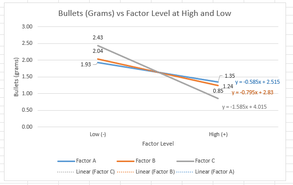
To determine the rankings of the factor that has the most to least significant impact on the mass of bullets, we must look at the factor with the steepest gradient. The greater the gradient coefficient, the more significant the factor affects the mass of bullets.
From the graph above, it can be shown that the ranking of the factors are:
Factor C: Power setting of the microwave is the most significant factor with the largest gradient coefficient of 1.585.
Factor B: Microwaving time is the next most significant factor with the second highest gradient coefficient of 0.795.
Factor A: Diameter of bowl is the least significant factor with the lowest gradient coefficient of 0.585.
Now that we have determine the rankings of the factors, it's time to determine the interaction effects. As previously mentioned, we have to do organize the data before we can plot the graphs as shown below.


Looking at the table, it can be shown that when factor A is low and factor B level increases from low to high, the mass of bullets decreases significantly from 3.12g to 0.95g. Similarly, as factor A is high and factor B level increases from low to high, the mass of bullets increases from 0.95g to 1.74g. However, the graph below shows a better way to analyze data.

To determine whether there are interaction between both factors, one have to also look at the gradient. The greater the difference in gradient, the larger the interaction between both factors. From the graph above, it can be seen that the gradient of both lines are different as one is positive which is 0.79 and the other is negative which is -2.17. Hence, there's a significant interaction between A and B. With A x B completed, it's time to repeat the same steps for A x C and B x C.
Calculating for A x C:

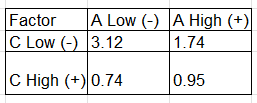
Looking at the table, it can be shown that when factor A is low and factor C level increases from low to high, the mass of bullets decreases significantly from 3.12g to 0.74g. Similarly, as factor A is high and factor C level increases from low to high, the mass of bullets decreases from 1.74g to 0.95g. However, the graph below shows a better way to analyze data.
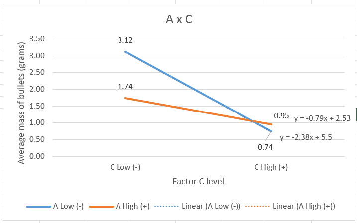
As previously mentioned again, to determine whether there are interaction between both factors, one have to also look at the gradient. The greater the difference in gradient, the larger the interaction between both factors. From the graph above, it can be seen that both lines are negative and of different values which are -0.79 and -2.38. Hence, there's a significant interaction between A and C. Lastly, it's time to repeat the steps for B x C.
Calculating for B x C:


Looking at the table, it can be shown that when factor B is low and factor C level increases from low to high, the mass of bullets decreases significantly from 3.12g to 0.95g. Similarly, as factor B is high and factor C level increases from low to high, the mass of bullets decreases significantly from 1.74g to 0.32g. However, the graph below shows a better way to analyze data.

As previously mentioned again, to determine whether there are interaction between both factors, one have to also look at the gradient. The greater the difference in gradient, the larger the interaction between both factors. From the graph above, it can be seen that both lines are negative and of different values which are -2.17 and -1. Hence, there's a significant interaction between B and C.
I have also attached the excel file for you to try out yourself!
Findings
Now that we have analyze our data, it can be seen that both runs 1,2,3,6 and runs 4,5,7,8 had the same trend! Hence, using either runs 1,2,3,6 or 4,5,7,8 will result in a similar result as they are both orthogonal! It's time to summarize our findings!
Increasing the factor levels for any factor will result in a decrease in the mass of bullets. As a result, there is a increase in popcorn yield as there are more edible popcorn.
The order for the most to least significant factor that impacts the popcorn yield is power setting of the microwave, microwaving time, diameter of the bowl.
For A x B: Increasing the diameter of the bowl and microwaving time will result in a significant interaction.
For A x C: Increasing the diameter of the bowl and power setting of the microwave will result in a significant interaction.
For B x C: Increasing the power setting of the microwave and microwaving time will result in a significant interaction.
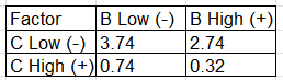
Now you might be wondering, how do we achieve the maximum popcorn yield from using the fractional factorial design. From the findings, we can deduce that we can set the power setting to the highest setting as it results in the largest decrease in mass of bullets. Additionally, we can deduce that the higher the interaction between two factors, the greater the impact on the popcorn yield. Since each factors had significant interaction with each other. It is important to set all factors to the highest level as it will allow us to achieve the maximum popcorn yield. This is also true as shown in the data above where setting all of the factor's level to high will result in the smallest mass of bullets of 0.32g.
Now that we have summarize our findings for fractional factorial design, let's move onto the next part of the blog!
Full vs Fractional
Full vs fractional? What's the difference? Going back to my point that design of experiments is able to save both resources and time, this statement is in fact true! This is because both full and fractional resulted in almost the same findings! Firstly, increasing the factor levels for any factor will result in a decrease in the mass of bullets. As a result, there is a increase in popcorn yield as there are more edible popcorn. Secondly, the order for the most to least significant factor that impacts the popcorn yield is power setting of the microwave, microwaving time, diameter of the bowl. Lastly, it can also be shown that A x B and B x C showed a significant interaction with each other!
However, there is a difference between full and fractional. There was a small interaction between A x C in full factorial design but a significant interaction between A x C in fractional factorial design! What does it mean and why? This means that using a larger set of data will result in a more accurate and reliable findings. This is because using a full factorial design eliminates any potential effects that are confounded that fractional factorial designs are sometimes not able to.
Does this mean you should use only full factorial design? No, even though full factorial design is able to eliminate any potential effects that are confounded, fractional factorial designs are still able to determine the most significant factor that affects the response variable. Additionally, using a fractional factorial design helps to save a lot of time and resources as shown in this experiment! Does this also mean that you should only use fractional factorial design? That's is a good question and I personally don't think so as it all comes down to context. When resources and time are limited, using a fractional factorial design will do just fine. However, when significant consequences such as safety risks or even death are involved, it's is crucial to take full factorial design as the primary choice as undetected interaction effects could lead to catastrophic failures.
Now that we have compare both full and fractional factorial design, let's move onto the next part of the blog!
Final Reflections
As we come near to the end of the blog, there are some learning points that I would like to share with you.
The first learning point is the importance of excel. Initially, I didn't expect myself to be using a lot of excel while doing this practical and tutorial. Even though I have learned how to use excel from one of my module in polytechnic foundation programme. This topic has challenged my excel skills. This is because I forgot how to do simple things such as creating graphs or even adding the equation line into the graph. As a result, I had to revise some of my work back in 2022 to relearn how to create graphs again. Hence, I have learned the importance of excel and I will not take it for granted.
The second learning point is the importance of organizing my work. This is because even though there were only 1 data set. There were many different workings and graphs to be calculated. As a result, it can be quite messy finding the graphs or calculations that I need. As a result, I used this opportunity to create two different sheets to separate the assignment into half which is full and fractional factorial design. This is important so that my graphs and calculations are reliable and accurate while being efficient. Hence, this practical and tutorial lesson has taught me the importance of organizing my work.
The third learning point is the importance of design of experiment. Initially, I did not realize how useful it could be as it could save time and resources. Additionally, I was also surprised to learn that I had use it for one of my practical modules last year. However, this tutorial and practical lesson has taught me the correct method of using design of experiments effectively and efficiently. This will be very helpful in the future as someone who wishes to pursue a career in the research and development field.
The final learning point is the trade-offs when using design of experiments. As previously mentioned, even though full factorial design is able to eliminate any potential effects that are confounded, fractional factorial designs are still able to determine the most significant factor that affects the response variable. Additionally, using a fractional factorial design helps to save a lot of time and resources as shown in this experiment. When resources and time are limited, using a fractional factorial design will do just fine. However, determining when to use full or fractional factorial design all comes to context. When significant consequences such as safety risks or even death are involved, it's is crucial to take full factorial design as the primary choice as undetected interaction effects could lead to catastrophic failures. Hence, I have the learned the trade-offs when using design of experiments.
With that, it is time to wrap my third blog on chemical product design. I had an amazing time writing this blog and learning the advantages and disadvantages of using design of experiments. I hope you had a great time reading a not to worry there are more coming soon. But for now, see you next time. Bye bye!


Comments